
This past weekend, Brett and I flew from Fairbanks to Anchorage and back; along the way, I pointed out Devils Canyon on the Susitna River as it passed below. “I listened to the most unbelievable podcast about this canyon and an airplane!” Brett told me, and proceeded to sketch in the plot while withholding the details to avoid spoiling the ending.
When we returned home that evening, as I continued making the edits to the Nenana River map as suggested to me by Bill Overington (aka Buckwheat), I listened to the podcast Brett had described – only to realize that the Devils Canyon podcast was about a paddling expedition gone wrong for Bill!
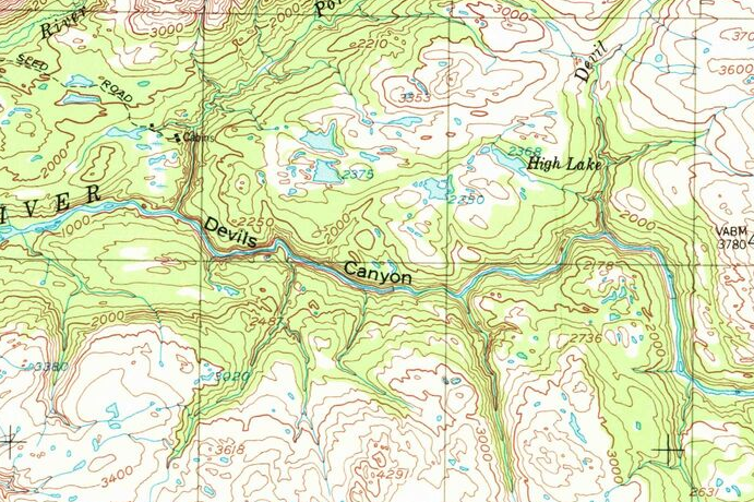
I now interrupt my regular Nenana River programming to give you this: a Devils Canyon map of the Susitna River, with or without labels.
The Devils
Devils (not Devil’s) Canyon is one of those places that, even without knowing anything about whitewater paddling, if you have been exposed to any cross-section of life in Alaska, you know it is a big deal.
First, it is considered part of the Alaska Triple Crown (along with the Grand Canyon of the Stikine River and Turnback Canyon of the Alsek River) not only because of Class V+/VI rapids, but add in the long swims, glacial water, and remote location, to make the stuff of legends – such as those told by Bill Overington and his friends. Listen to Part 1 and Part 2 of their kayaking story from 1995. And if you think the story about the plane in Devils Canyon is unbelievable, there is also the one about Alaska flying legend Don Sheldon.
In my mind, the Susitna River – specifically Devils Canyon – is also tied to another story of legendary status in Alaska. In the late 1890’s, a gold prospector named William Dickey traveled throughout the Susitna River drainage. Dickey’s tie to Devils Canyon came when his party traveled up the Susitna River but could not find a way to portage the canyon, so had to turn back. Before they left the area, they made their indelible mark on a rock at Portage Creek, which is still there to this day.
In addition to leaving a physical mark on the land, Dickey’s trip set the stage for a propaganda push to rename the Denali massif to “Mount McKinley”, even though Denali had been known by Alaska Natives in the region by the Athabaskan dialect variants of “Denali” for thousands of years.
In a testament to the power of maps, one of the main reasons Dickey’s preferred name stuck so well was because in 1896, he was one of the first people to publish a map depicting the Denali massif in a popular, widely-distributed, English-language periodical. His Susitna River map not only helped fix a name in the mind of the masses of the United States, but his map was also the first English map with an estimated height of the Mountain.
Thankfully, the State of Alaska formally returned to the name “Denali” less than 100 years later; the Federal government eventually followed suit, formally recognizing the original name in 2015. It is my pleasure (and day job) to enforce this correction on any map I can.
While we are on the subject of names, I will mention that one of my favorite things about Alaska is how many Native place names remain in place, such as “Susitna”.
On the other hand, the name of “Devil Creek” was in Orth’s Dictionary of Alaska Place Names as a local place name in the 1950’s, but with no explanation and no mention of a “Devils Canyon”.
The name “Devils Canyon” does not appear on any USGS 1:63,360 Topographic maps until the 1970 edition of a 1:250,000 map.
The earliest reference I can find to a Devil Canyon in that area is a US Fish and Wildlife report from 1952 regarding the proposal of the Bureau of Reclamation’s “Devil Canyon” and Denali damsite.
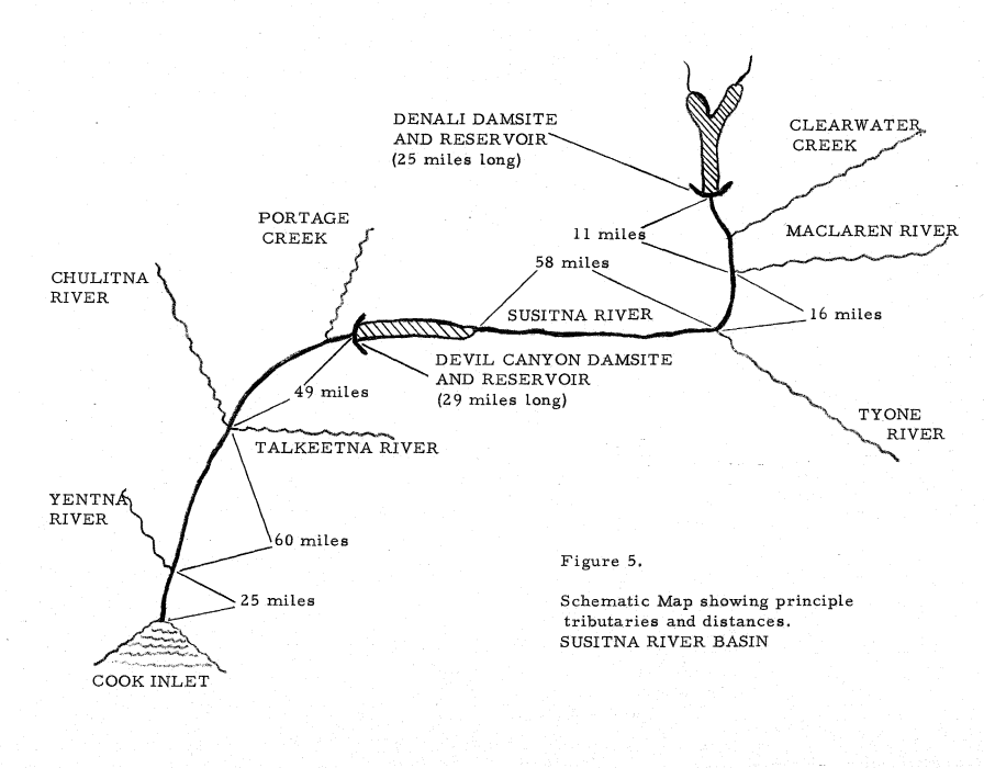
Which leads into another reason that part of the Susitna River is somewhat well-known: Proposed hydroelectric projects for the area have been studied in the 1960’s and the 1980’s and the early 2010’s. Most recently, support faded in 2014 when the funds for the studies dried up, but the subject continues to be floated in certain circles from time to time. The project as it currently stands would build a 705 foot tall dam and a 44 mile long reservoir on an anadromous salmon stream.
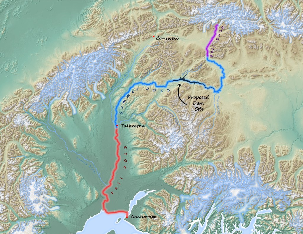
In 2012/2013, a former co-worker of mine, Chris Dunn, paddled the entirety of the Susitna River alone, portaging parts of Devils Canyon. He documented his 300+ mile journey and wrote an very detailed, very interesting 3-part series for the Ground Truth Trekking blog. My interest in his travels led me to make the map that accompanies his story (my first real map for “hire” – be kind!).
The Details
Coming back to the present, these were all the things that I thought about this past weekend as I flew over the canyon, which was less impressive in the winter at 10,000′ mean sea level. Which got me to thinking…
Many of the maps I make are designed to be descriptive, with so many vectors as to feel cartoonish. I knew that I wanted a Devils Canyon map that was mostly decorative but hyper-realistic for this map to focus on the terrain itself. Thankfully, a former National Park Service Harpers Ferry Center cartographer, Tom Patterson, has outlined some concepts of cartographic realism that I tried to follow while making this map.
Here are the ingredients I used to make my realistic map:
- Hillshade (with multipoints and collar extents)
- Curvature (i.e., concavity/convexity)
- Slope (with red color gradients)
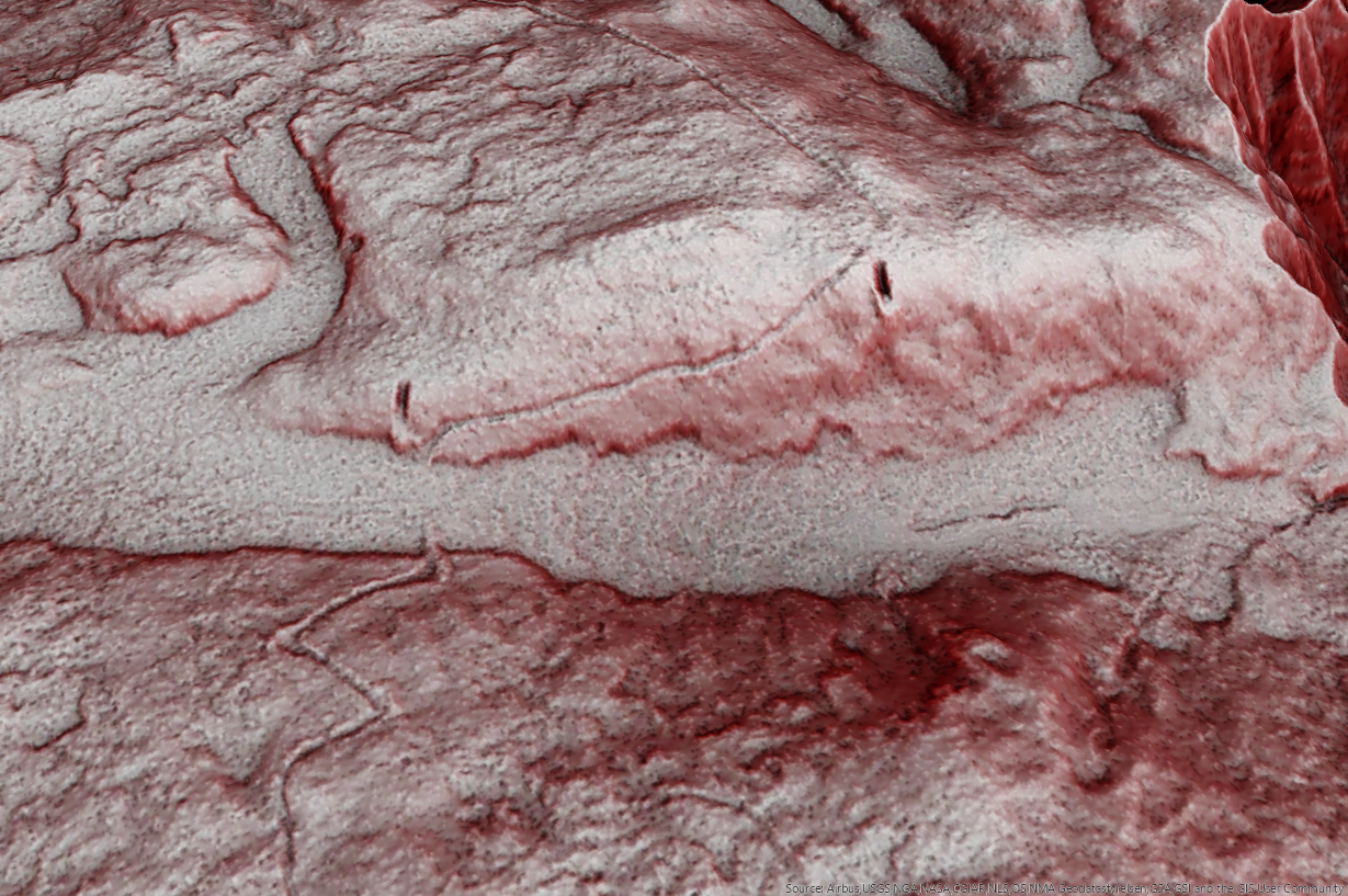
- Detrended elevation model (with red color gradient)
- Imagery (masked and blended with hillshade)
Terrain
The public has access to LiDAR and aerial imagery from the 2011 Mat-Su Borough project, so I downloaded the Bare Earth DEM and the imagery covering the canyon. Given that the best statewide digital elevation model is roughly 5 meter GSD and the canyon in some places is less than 30 meters wide, I was grateful for the higher resolution DEM for defining the tight, vertical canyon.
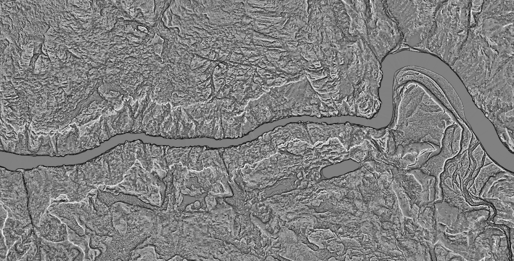
My idea behind incorporating hillshading was to add depth to the map by creating shadows while avoiding the harsh lighting of single point hillshading. Although John Nelson often creates the same effect with his layers upon layers of hillshades (and hillshades of slopes!), I prefer something that requires a little less thought on my part. That is where the Sky model from the Esri created toolbox Terrain Tools comes in.
A sky model is a “quantitative representation of natural luminance of the sky under
various atmospheric conditions” with luminance defined as “the flux density of light emitted from a point in a direction. Luminance can come from the sky or from the ground. ‘Illumination’ is a pattern of luminance from the sky.”1 In other words, not only does it matter where the sun sits on the horizon, but it also matters how the light scatters (both coming in and going back out) throughout the sky.
Before I began the process, I could see shadows cast by the sun in the 2011 imagery. Although I knew that these shadows would not affect the lidar, if I hoped to match the imagery further on in the process, I would need to match the light source in the model to the lighting of the image. Using a sun calculator, I determined the sun’s azimuth (direction) and elevation (angle above the horizon) for that area to the date the imagery was captured.
I then used that information in the Sky Luminance program that comes with the Terrain Tool. The Sky Luminance program creates a dome meant to represent the sky, and then allows a user to choose from a bunch of different sky models, as well as alter the light source’s azimuth and elevation. Once the user is happy with the model and light source location, the program will then create a lot of points meant to represent the direction of illumination, weighted by algorithms determined from the sky model the user chose. The user then saves the attributes for each point in a text file.
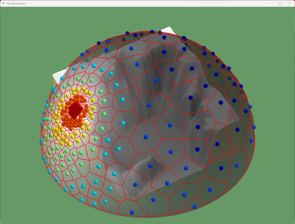
distribution:  CLEAR
sun elevation: 45
sun azimuth:   180
sample points: 250

Format of sample points: azimuth,elevation,weight (weights sum to 1.0)

180,45,0.000464042
177,41,0.000639647
185,42,0.000911906
176,47,0.000988032
......
I eventually went with a turbid sky model, that cast subtle shadows and avoided the “waxy” look I associate with harsh and single point sky models.
While I was at it, why not apply some 3D Relief map in to add to the realism, in a Sean Conway style? I followed some of the steps outlined by John Nelson here, but then threw in a little extra, such as using a constant value that was slightly above the lowest part of the river. This allowed most of the canyon to appear to be below the edge of the map. I also ran Extract by Mask to add the title box into the elevation raster so that it would look a bit “baked” into the hillshade.
Curvature
I’ve been considering updating or revisiting the Red Relief Image Map post I made a few years back, mainly to point out one more aspect to the RRIM method that I feel can be mimicked using other geoprocesses. RRIM uses a combination of an openness index with a slope gradient, but it is still ultimately for display, not an analysis. There are now two features in ArcGIS Pro that can mimic the RRIM display.
The first we will talk about is Surface Parameters tool (previously the more simplified Curvature tool).
This tool will create a raster with cells indicating convex and/or concave areas to add some realism to my hillshade. The Profile output of the tool emphasizes the concavity/convexity as a concept of flow down a slope, while the Tangential output of tool emphasizes the concavity/convexity across the slope; the first creates an appearance of terraces while the latter an appearance of ridges and valleys. A mean curvature output produces the same effect as one would achieve through blending the Profile with Tangential outputs. I used a large neighborhood distance and an adaptive neighborhood to reduce noise in the flatter areas.
Profile Curvature 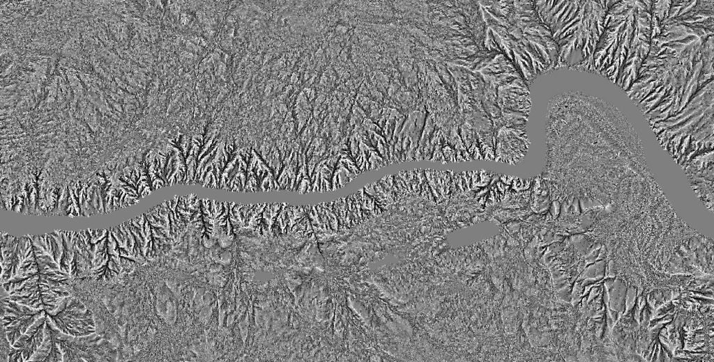
Tangential Curvature 
Mean Curvature
From there, combining the curvature with slope is the same as an RRIM method (see below in Blends). But why not also add it to a hillshade? I was so proud of myself for thinking to use this tool in combination with hillshade, only to discover (or maybe rediscover) that it was already a well-established method. The veritable Aileen Buckley describes it here.
Tom Patterson achieved a similar look as curvatures combined with hillshades through a method called “texture shading”, using a software created by Leland Brown. This method was designed to emphasize ridges and canyons, and also uses differential geometry.
When I first dabbled in using this Terrain Texture about a decade ago, I tested it out on a dataset for Devils Canyon, of course. Tom was very helpful in assisting me as I struggled to learn the command line, but as Tom says himself in the blog, the real magic happened in Adobe Illustrator/Photoshop, and I have yet to become proficient in that software suite.
Blends
The second part of RRIM that can be mimicked is through blend modes. It isn’t exactly clear in the original RRIM paper how the slope gradient and openness index was “merged”, but it is clear that some kind of blend mode or bivariate symbology was used. The relatively new Blend modes in ArcGIS Pro allow me to accomplish that same look by blending slope gradient and the curvature raster.
But blends also blend nicely into the rest of the map.
First, I applied blends to incorporate the hydrological features from the map, since the vectorized features took away from the realism. Also, I wanted the rapids in the Canyon to be displayed without using vectors. I then also applied a blend to let the hillshade that I had created using the Skymodel tool shine through.
Yet, even with the hillshade, curvature, and slope, I still wasn’t able to get canyon to pop like I wanted. Essentially, I needed to create a raster with values that were relative to the elevation from the centerline of the river up the banks. I settled on a “Height Above Nearest Drainage” model from Thomas Dilts’ Topography Toolbox. This allowed me to display the depth of just the river with a red gradient.
Finishing Touches
As usual, I finished it up by slapping it with some stuff I stole from John Nelson. I’m the kind of person who worries that people will think I take myself too seriously if I use serifs, but I felt like this map desired not just one serif font, but two. I’m serious.
And finally, I’m dedicating the version of the map with a few places labeled to thank Buckwheat, Q, Mikey K., Jerry, and Connie for sharing their story. I’m glad it had a happy ending.
- Patrick J. Kennelly & A. James Stewart (2014) General sky models for
illuminating terrains, International Journal of Geographical Information Science, 28:2, 383-406,
DOI: 10.1080/13658816.2013.848985 ↩︎

You must be logged in to post a comment.